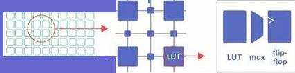
FPGA based Digital World
Welcome to FPGA based Digital World.
Signal processing is much important. |
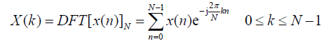
Discrete Fourier Transform(DFT)
For a signal series x(n) with M points (0 to M-1), its DFT is defined as
let 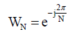 , its DFT and IDFT(inverse discrete Fourier transform become
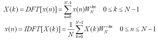
or
x(n)<--DFT/IDFT--> X(k)
The above transform can be explained as below.
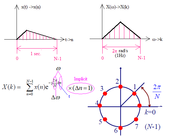
X(k) is regarded as the N-point sampling of the Fourier transform of x(n)(0 to 1s).
Note:
(1) X(k) is complex, while x(n) is real.
(2) X(k) is not the spectrum of x(n), but the sampling of one period of the spectrum(explained below).
(3) If the points of x(n) are sampled with sampling frequency fs from x(t), then the actual freqeuncies of X(k) should be multiplified by fs.
(4) If x(k) is real, then the Fourier transform is corjugate symmetric, which implies that the real part and the magnitude are both even functions and the imaginary part and phase are both odd functions. Thus for real-valued signals the Fourier transform need only be specified for positive frequenciesbecause of the conjugate symmetry.
(5) Whether or not a sequence is real, specification of the Fourier transform over a frequency range of 2π specifies it entirely.
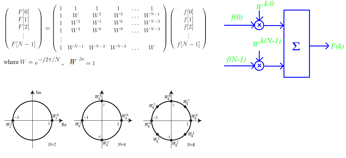
DFT can also be writen in matrix form as
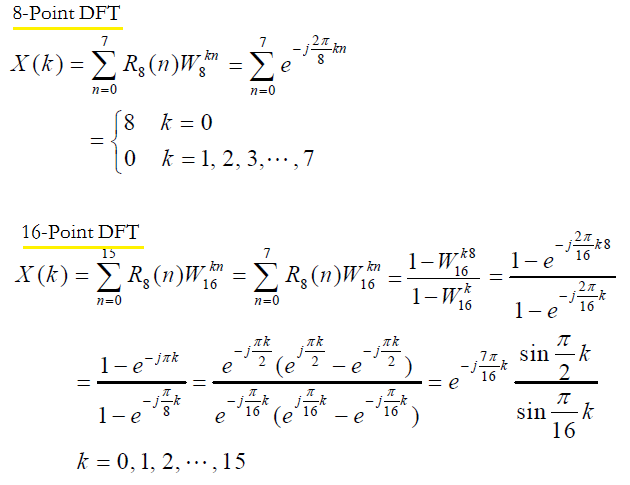
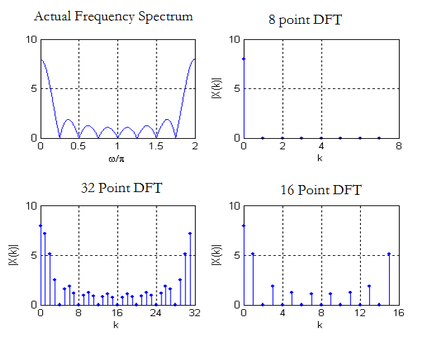
[Example] x(n) is a 8-point rectangular function, defined as below, calculate its discrete Fourier transform with N=8 and 16.
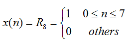
And the solution is shown below.
Basic Rules
Below basic rules need to be remembered to understand the transition from FT to DFT.
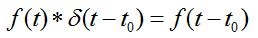
Rule 1: The convolution of function f(t) with a pulse function, is a mirror of f(t) to the pulse position(both in time or frequency domain), i.e.,
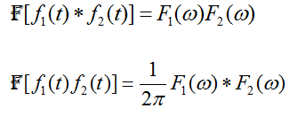
Rule 2: The multiplication of two functions in one domain corresponds to the convolution of the twos in another domain, i.e.
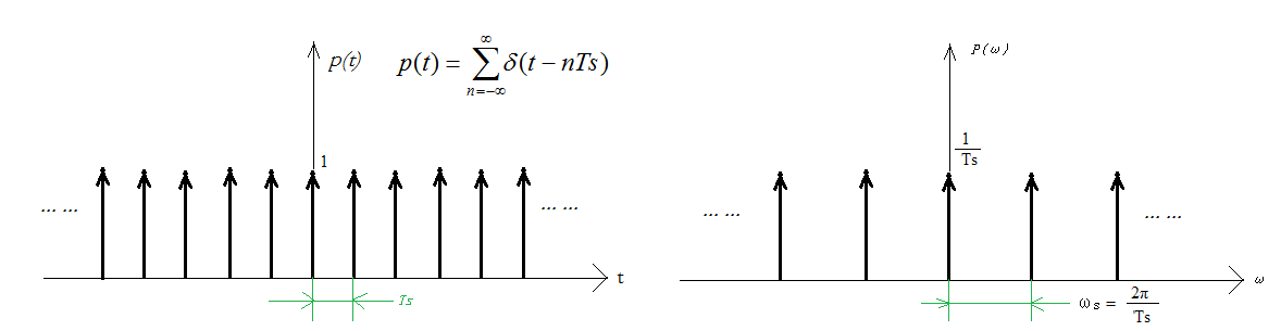
Rule 3: The sampling funciton is a series of pulse functions and its Fourier transform is also a series of pulse functions.
From FT to DFT
An aperiodic signal is continous in time domain, and its Fourier transfrom in frequency domain is also continous.From FT to DFT insists of several steps, as shown below.
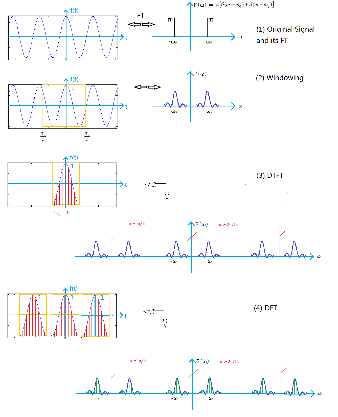
(1) FT
Taking below time-domain function as the example
f(t)= cos(ω0t)
Its Fourier transform is two δ functions at -ω0 and ω0, which is shown on the right side of (1).
Note: the signal is continuous in both time and frequency domain.
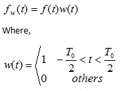
(2)Windowing
The original signal is infinite, so it must be windowed to a finite range.And it causes leakage in some cases(as depicted below).
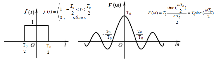
Rectangular window in time domain is used in this case, whose Fourier transform is a sinc funcition(as shown below).
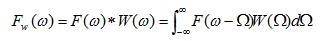
Windowing is equal to multiply the rectangular function with the signal,which causes the convolution in frequency domain(rule 2). And according to rule 1, the result is the mirroring of sinc function to -ω0 and ω0, as shown on the right side of (2).
The f(t) now becomes
And F(ω) becomes
Note: The signal is still continuous in both time and frequency domain.
(3) DTFT(Discrete Time Fourier Tranform)
The signal is sampled in time domain with sampling pulses, and it's a multiplication of the sampling function p(t) and the signal f(t).--> Convolution of F(ω) and P(ω) in frequncy domain(Rule 1).--> F(ω) is mirrored to P(ω)(Rule 2), as shown in the right part of (3).
Note: The signal is discrete in time domain, but still continuous in frequency domain.
(4) DFT(Discrete Fourier Tranform)
The signal is sampled in frequency domain with sampling signal, and causes the signal to be mirrored in time domain, as shown in (4).
Note: The signal is now discrete in both time and frequency domain.
[Example] A continuous signal is shown below, and the sampling frequency is fs=4Hz, so the sampled series are f(n) are: 8,4,8,0.
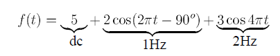
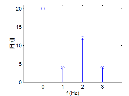
The F(n) is calculated as
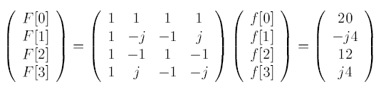
And the amplitude spectrum is shown.
DFT Properties
1 Linearity
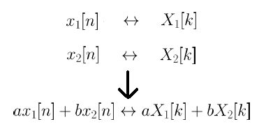
If the two sequnces are of different lengths, append zero(s) to the shorter sequence to makethem with the same duration.
2 Circular Shift of Sequence
x(n) (n=0 to N-1)is to extended to a periodic sequence with period of N as,
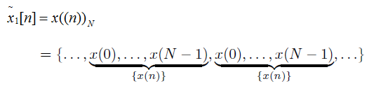
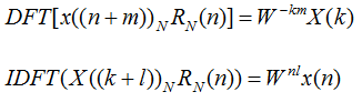
Then the cirular shift is defined as
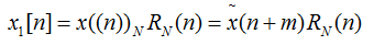
wher RN is a N-point rectangular sequence.
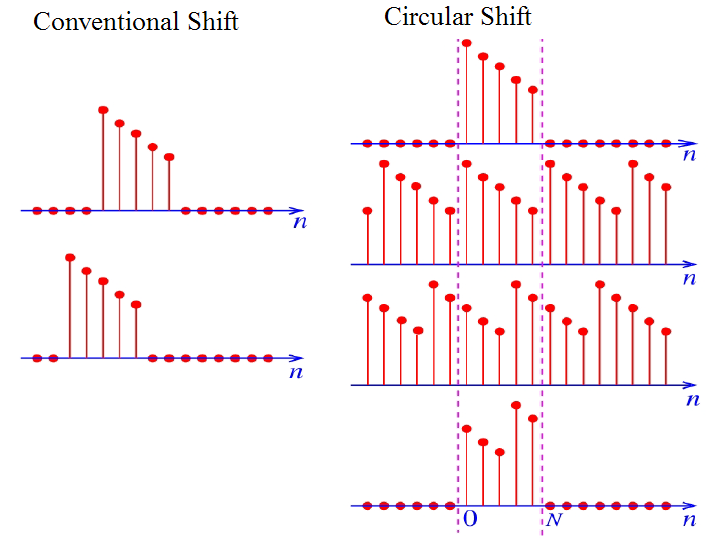
The relation of the cirular shifted sequence to the original one is as below.
3 Duality
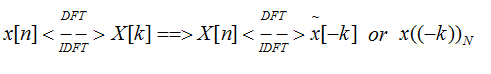
4 Symmetry
Refer to the symmetry in DFS.
5 Circular Convolution
Refer to the circular convolution in DFS.
DFT Errors
DFT is only an approximation to FT since it provides only for a finite set of sequence and frequencies, and it causes two main errors: aliasing and leakage.
1 Aliasing: due to time-sampling rate limitation
2 Leakage
The continuous Fourier transform of a periodic waveform requires the integration to be performed over the interval -∞ to ∞ or over an integer number of cycles of the waveform. If the DFT is compelted over a non-integer number of cycles of the input signal, then leakage occurs.
Window functions taper the samples towards zero values at both endpoints, and so there
is no discontinuity (or very little) with a hypothetical next period. Hence the leakage of spectral content away from its correct location is much reduced.
Different Fourier Transforms
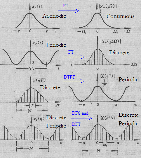
The relationship between continuity and periodicity is summarized as below.
Continous in one domain --> Aperiodic in another domain
Discrete in one domain --> Periodic in another domain
Below is a detailed table.
| Type | Time Domain | Frequency Domain | Comment |
| FT | Aperiodic, Continuous | Continuous, Aperiodic | |
| FS | Periodic, Continuous | Discrete, Aperiodic | |
| DTFT | APeriodic, Discrete | Continous, Periodic | |
| DFT | Periodic, Discrete | Discrete, Periodic |
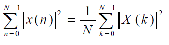
Parseval's Theroem in DFT
DFT in Matlab
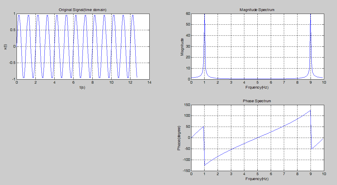
An example to calculate DFT in Matlab is shown below.
%--------------------------------------
% Example of cosine wave spectrum
% -------------------------------------
% Overal Paramters
f0 = 1; %frequency of the cosine wave, Hz
fs = 10; %Sampling frequency, in Hz
N = 128; %Sampling Number
% Sampling
n = 0:N-1; %discrete sampling number series
t = n/fs; % discrete sampling time, in sec.
% for calculating function values
Xt = sin(2*pi*f0*t); %discrete samples
% Call FFT(DFT) function in matlab
Xf = fft(Xt,N); % FFT, same as DFT, but fast
Frq= (0:N-1)'*fs/N; % Corresponding frequency array
% Calculate magtitude and phase of the FFT
Xf_Mag = abs(Xf);
Xf_Phase = angle(Xf)*180/pi; % in degree
% Calculate Power
Xf_Power = Xf_Mag.^2;
% Plot original signal in time domain
figure(1);
subplot(221);
plot(t, Xt);
xlabel('t(s)');
ylabel('x(t)');
title('Original Signal(time domain)');
grid;
% Plot Manitude in frequency domain
subplot(222);
plot(Frq, Xf_Mag);
xlabel('Frquency(Hz)');
ylabel('Magnitude');
title('Magnitude Spectrum');
grid;
% Plot Phase in frequency domain
subplot(224);
plot(Frq, Xf_Phase);
xlabel('Frquency(Hz)');
ylabel('Phase(degree)');
title('Phase Spectrum');
grid;
And the running result is as follows.
| Altera/Intel | Xilinx | Lattice | Learn About Electronics |
| MircoSemi | Terasic | Electric Fans |
| All rights reserved by fpgadig.org |